Kalman Filter: An Introduction

Kalman Filter is a widely used algorithm for estimating the state of a system based on noisy observations. It was developed by Rudolf E. Kálmán in the early 1960s and has since found numerous applications in various fields such as engineering, robotics, finance, and more. In this blog post, we will discuss the basics of Kalman Filter, including its history, principles, and applications.

What is Kalman Filter?

Kalman Filter is a recursive algorithm that estimates the state of a system over time based on a sequence of observations that are corrupted by noise. It uses a mathematical model of the system dynamics and measurements to estimate the true state of the system. The basic idea behind Kalman Filter is to use the available data to infer the state of the system and to update this estimate as new data becomes available.

History of Kalman Filter

The development of Kalman Filter was motivated by the need to solve a problem in control theory known as the linear quadratic regulator (LQR) problem. The LQR problem involves finding a control policy that minimizes a quadratic cost function while ensuring that the system remains stable. Rudolf E. Kálmán, a Hungarian-American mathematician and electrical engineer, proposed a solution to this problem in 1960 using a recursive algorithm that estimated the state of the system based on noisy measurements.

How does Kalman Filter work?

Kalman Filter works by maintaining a probabilistic estimate of the state of the system over time. This estimate is represented as a Gaussian distribution with mean and covariance, which are updated recursively based on the new observations. The state of the system is assumed to follow a linear dynamic model with Gaussian noise, and the observations are assumed to be linearly related to the state with Gaussian noise. The Kalman Filter updates the estimate of the state based on a two-step process: prediction and update.

Prediction step :

In the prediction step, the Kalman Filter uses the current estimate of the state and the state transition model to predict the state of the system at the next time step. The predicted state is represented as a Gaussian distribution with mean and covariance, which are computed using the following equations: x̂_k|k-1 = F_k x̂_k-1|k-1 + B_k u_k + w_k P_k|k-1 = F_k P_k-1|k-1 F_k^T + Q_k

where:

x̂_k|k-1 is the predicted state of the system at time k given the observations up to time k-1.

F_k is the state transition matrix that describes how the state evolves over time.

B_k is the control input matrix that describes how the control input affects the state.

u_k is the control input at time k.

w_k is the process noise, which is assumed to be Gaussian with mean 0 and covariance Q_k.

P_k|k-1 is the predicted covariance of the state estimate at time k. In the update step, the Kalman Filter uses the predicted state and the observation model to update the state estimate based on the new observation. The updated state is represented as a Gaussian distribution with mean and covariance, which are computed using the following equations:

MATLAB CODE FOR KALMAN FILTER

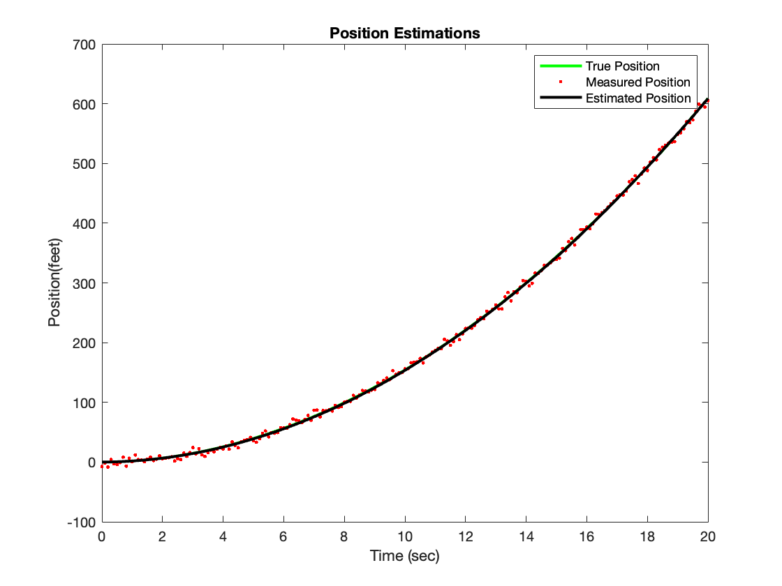
Here is the solution of the movement of an object with a constant acceleration by using Matlab

Let the position of a vehicle be measured at 5 feet (with a standard deviation) acceleration of 3 feet/sec2 and a measurement noise of 0.1 feet/sec2 (a standard deviation). Since the position is measured every 5 seconds, let's try to estimate the position of this vehicle in the best way with the Kalman filter in 20 sec duration.

clc

clear

duration=20;

dt=0.1;

measnoise = 5; %position measurement noise (feet)

accelnoise = 0.1; %acceleration noise (feet/sec^2)

A = [1 dt; 0 1]; %transition matrix

B = [dt^2/2; dt]; %input matrix

C = [1 0]; %measurement matrix

x = [0; 0]; %initial state vector

xhat = x; %initial state estimate

Sz = measnoise^2; %measurement error covariance

Sw = accelnoise^2 \* [dt^4/4 dt^3/2; dt^3/2 dt^2];
P = Sw; %initial estimation covariance

%Initialize arrays for later plotting.

tpos = []; %true position array

poshat = []; %estimated position array

posmeasured = []; %measured position array

for t = 0 : dt: duration

%Constant acceleration

u = 3;

%Simulation

ProcessNoise = accelnoise * [(dt^2/2)*randn; dt\*randn];

x = A _x + B_ u + ProcessNoise;

%Measurement noise

MeasNoise = measnoise \* randn;

y = C \* x + MeasNoise;

%Estimation

xhat = A _xhat + B_ u;

Inn = y - C \* xhat;

s = C _P_ C' + Sz;

%Kalman gain

K = A _P_ C' \* inv(s);

%State estimate

xhat = xhat + K \* Inn;

%Estimation error

P = A _P_ A' - A _P_ C' _inv(s)_ C _P_ A' + Sw;

%values to plot

tpos = [tpos; x(1)];

posmeasured = [posmeasured; y];

poshat = [poshat; xhat(1)];

end

%Plotting

t = 0 : dt : duration;

figure;

plot(t,tpos,'g','LineWidth',2);
hold on

plot(t,posmeasured,'r.','LineWidth',2);

plot(t,poshat,'k','LineWidth',2);

title('Position Estimations');

xlabel('Time (sec)');

ylabel('Position(feet)');

legend('True Position', 'Measured Position', 'Estimated Position')

References

1. R. E. Kalman, "A new approach to linear filtering and prediction problems," Transactions of the ASME -- Journal of Basic Engineering, vol. 82, pp. 35-45, March 1960.
2. G. Welch and G. Bishop, "An introduction to the Kalman filter," Technical Report TR 95-041, University of North Carolina at Chapel Hill, 2006.
3. S. Särkkä, "Bayesian filtering and smoothing," Cambridge University Press, 2013.
4. A. Gelb, "Applied optimal estimation," The MIT Press, 1974.
5. D. Simon, "Optimal state estimation: Kalman, H infinity, and nonlinear approaches," John Wiley & Sons, 2006.